Subsetting Tool

The Subsetting Tool allows you to create scenarios of abiotic factors and search for accessions that can grow under these conditions. The tool considers only accessions that specify the coordinates of their collecting sites.

The tool uses a spatial resolution of approximately 5 km (a 5 by 5 km box near the equator), which means some accessions sharing the same pixel are grouped together in the analysis.

Agroclimatic indicators

The Subsetting Tool uses a set of agroclimatic indicators grouped into six categories. These indicators are calculated from long-term climate data spanning multiple decades.

Drought stress

• Total precipitation: Total monthly precipitation measured in millimeters (mm).
• Consecutive dry days: Maximum number of consecutive days with precipitation less than 1 mm.
• Number of days with water stress: Number of days per month in which the ratio between actual and potential evapotranspiration (ERATIO) is less than 0.5. ERATIO is calculated following a simple water balance model.

Flood stress

• Extreme daily precipitation: 95th percentile of precipitation per month measured in millimeters. This indicator shows the highest values of precipitation.
• Number of days with flooding: Number of days per month in which the ratio between actual and potential evapotranspiration (ERATIO) is greater than 0.5.

Heat stress

• Average minimum temperature: Average monthly minimum temperature, measured in degrees Celsius.
• Average maximum temperature: Average monthly maximum temperature, measured in degrees Celsius.
• Average VPD: Monthly average vapor pressure deficit.
• Number of days with high VPD: Number of days per month for which the vapor pressure deficit is greater than or equal to 4 kPa.

Photoperiod indicators

• Mean solar radiation: Monthly average of solar radiation measured in W/m2.
• Julian day length: Average daylight hours per month.

Soil indicators

• Bulk density: Bulk density averaged over the top 60 cm of soil, measured in Cg/cm3.
• Cation exchange capacity: Average cation exchange capacity over the top 60 cm of the soil, measured in mmol(c)/kg.
• Type of soil texture: Qualitative variable indicating soil classes taken from USDA soil taxonomy.
• Organic carbon content: Organic carbon content averaged over the top 60 cm of soil, measured in dg/kg.
• pH: Soil pH averaged over the top 60 cm of soil, measured at pH times 10.
• Salinity: Qualitative variable indicating soil salinity class taken from FAO.

Crop-specific indicators

The crop-specific indicators are available only for the crops listed in the table below. These indicators use temperature cut-off points specific to each crop.

• Number of days with high temperatures: Number of days per month in which the maximum temperature exceeds the maximum temperature supported by the crop.
• Number of days with low temperatures: Number of days per month in which the minimum temperature is below the minimum temperature supported by the crop.
• Number of days with optimal temperatures: Number of days per month in which the average temperature oscillates between the optimum temperatures for crop growth.

Crop	Heat stress	Cold stress	Optimum
Beans	Tmax > 25.6	Tmin < 13.5	17.5 < Tmean < 23.1
Cassava	Tmax > 45	Tmin < 15	22 < Tmean < 32
Banana	Tmax > 35	Tmin < 15	24 < Tmean < 27
Wheat	Tmax > 32	Tmin < 10	18 < Tmean < 25
Maize	Tmax > 28	Tmin < 15	28 < Tmean < 29
Potato	Tmax > 24	Tmin < 4	12.4 < Tmean < 17.8
Sweet potato	Tmax > 35	Tmin < 15.5	20 < Tmean < 32
Rice	Tmax > 40	Tmin < 13	20 < Tmean < 35
Barley	Tmax > 36	Tmin < 3	18 < Tmean < 24
Sorghum	Tmax > 17.8	Tmin < 39.1	26.7 < Tmean < 37.4
Pearl millet	Tmax > 50	Tmin < 13.3	12.4 < Tmean < 17.8
Cowpea	Tmax > 50	Tmin < 15	20 < Tmean < 35
Yam	Tmax > 40	Tmin < 20	25 < Tmean < 34
Soybean	Tmax > 37	Tmin < 14	25 < Tmean < 28

Table 1: Temperature cut-off points by crop

Accessing the Subsetting Tool

The Subsetting Tool is accessible only to registered Genesys users. Please log in first.

Step 1: Apply passport filters

Once logged in to the Genesys database, first filter for accessions of interest based on their passport data.

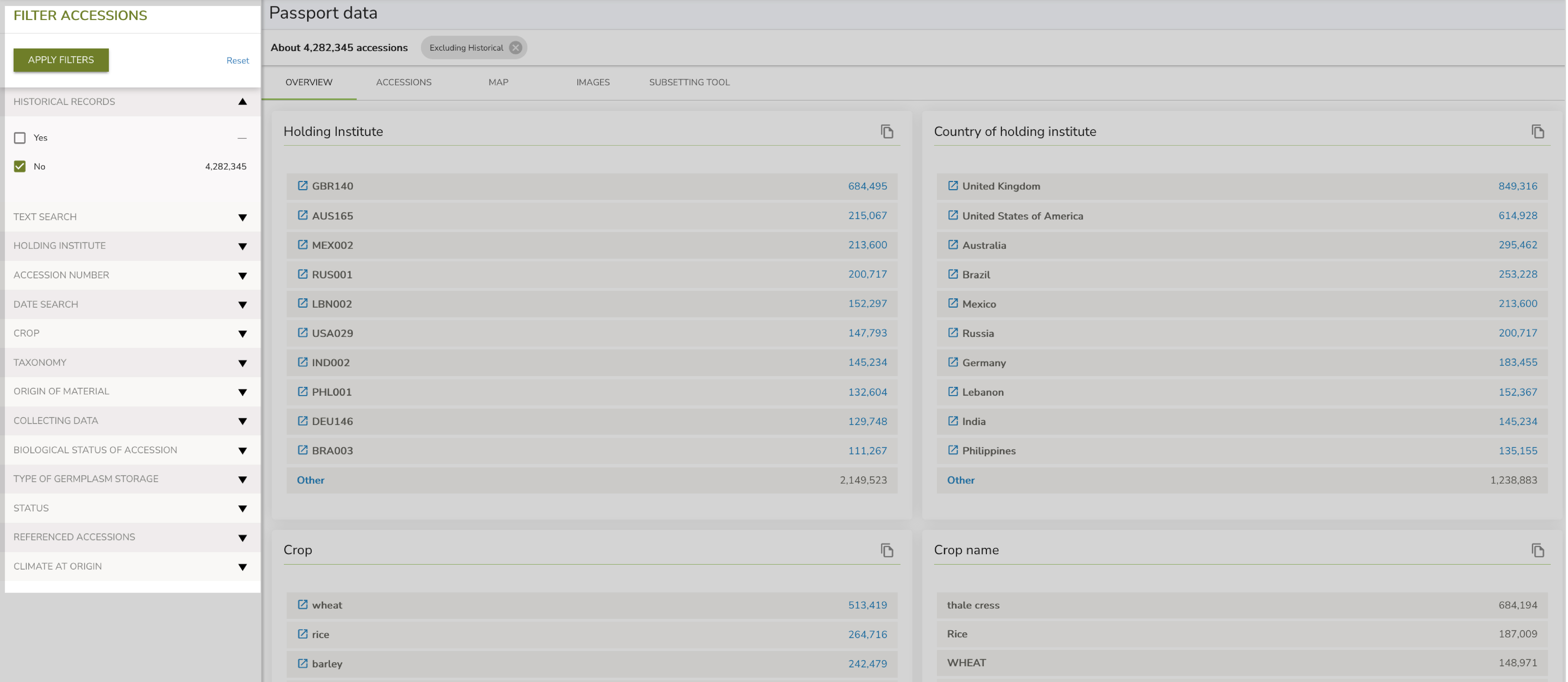
Figure 1: Applying filters by passport data

Genesys allows filtering of accessions in multiple ways:

• Text search: Search accessions containing text in any field.
• Holding institute: Search by the institute code of the institute holding the accessions.
• Accession number: Search by accession number.
• Crop: Filter by the crop of interest.
• Taxonomy: Filter by taxonomy classification.
• Origin of material: Filter by origin country.
• Collecting data: Filter by collecting date, number, mission, or location.
• Biological status: Filter by wild, weedy, landrace, breeding material, improved cultivar, GMO, or other.
• Type of germplasm storage: Filter by seed collection, field collection, in vitro collection, cryopreserved collection, DNA collection, or other.
• Status: Filter by availability for distribution, georeferencing data, inclusion in the Multilateral System, backup in Svalbard, or AEGIS status.
• Climate at origin: Filter accessions considering climatic patterns of their collecting sites.

Step 2: Open the Subsetting Tool

After applying your passport filters, click the APPLY FILTERS button and then navigate to the SUBSETTING TOOL tab.

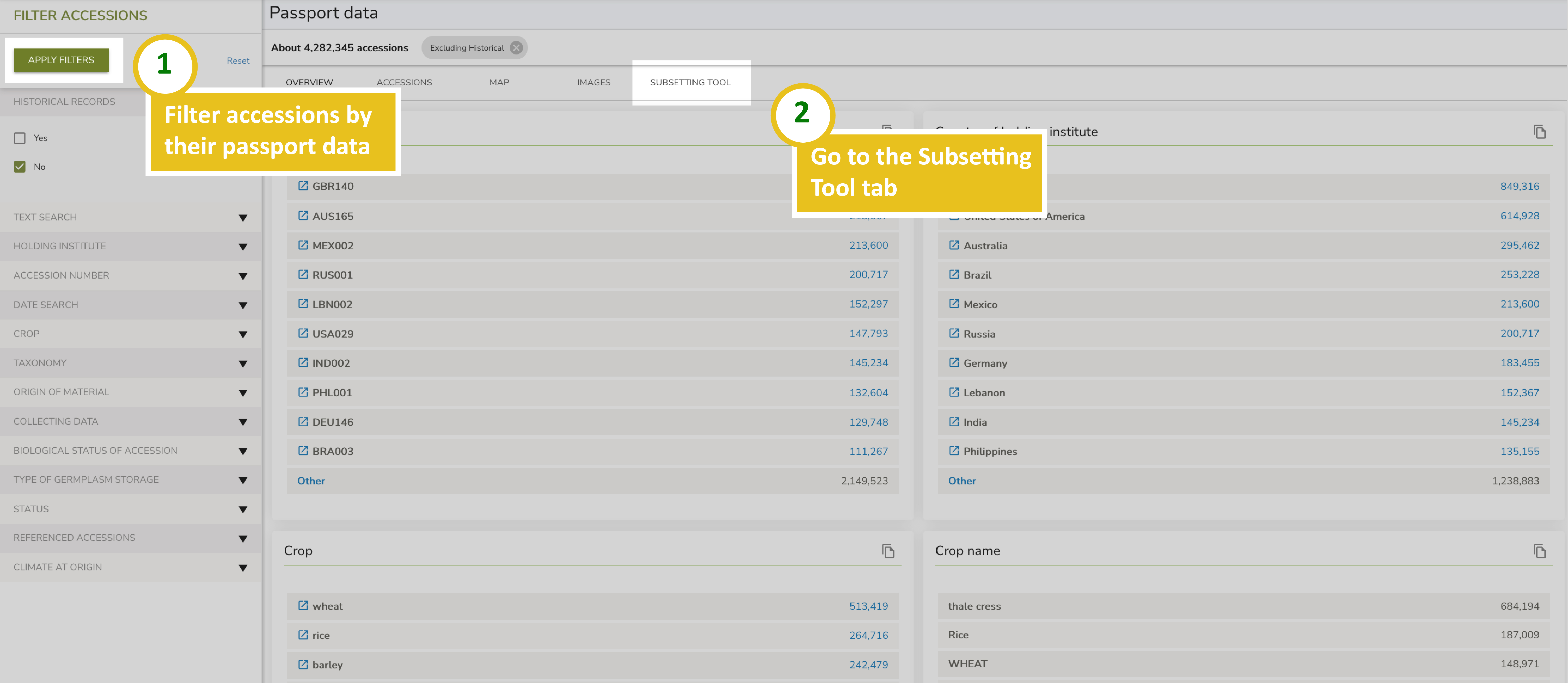
Figure 2: Steps to apply filters and open the Subsetting Tool

tip

Always click APPLY FILTERS before entering the Subsetting Tool. Skipping this step causes the subsetting tool to ignore your previous selection and consider all accessions in Genesys.

Using the Subsetting Tool

The tool has two modes: basic indicator selection and advanced indicator selection. The basic mode allows selection of indicators with general parameters. The advanced mode provides more control, letting you specify a range of values for each indicator.

Basic mode example: Finding beans for a Colombian farm

Imagine a Colombian farmer growing beans who wants to request seeds from the genebank. The farmer knows his field has high rainfall and low temperatures.

1. Apply a passport filter for beans as the crop before entering the Subsetting Tool.

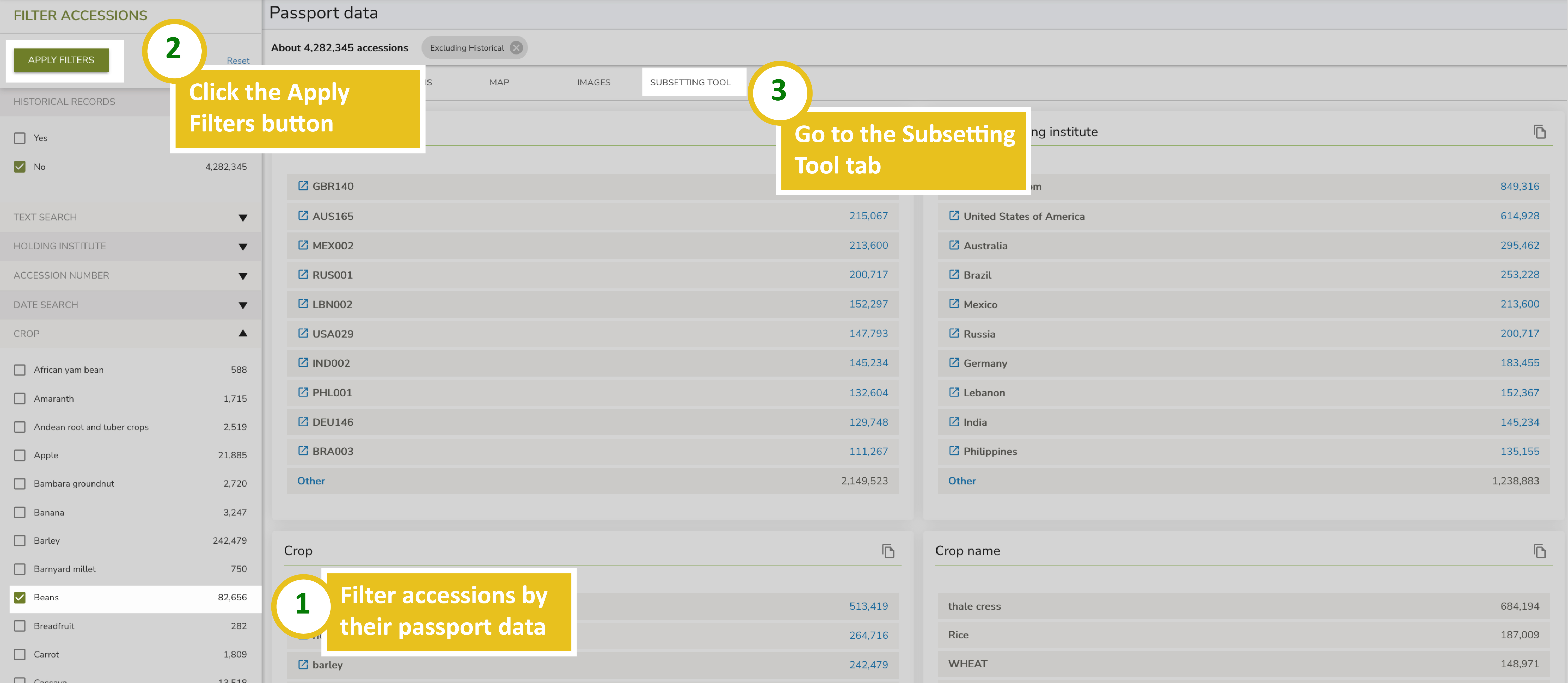
Figure 3: Filtering beans accessions based on passport data before entering the subsetting tool

2. In the Subsetting Tool, select indicators matching the field conditions. For example, choose flood stress indicators (high rainfall) and crop-specific indicators for low temperatures.

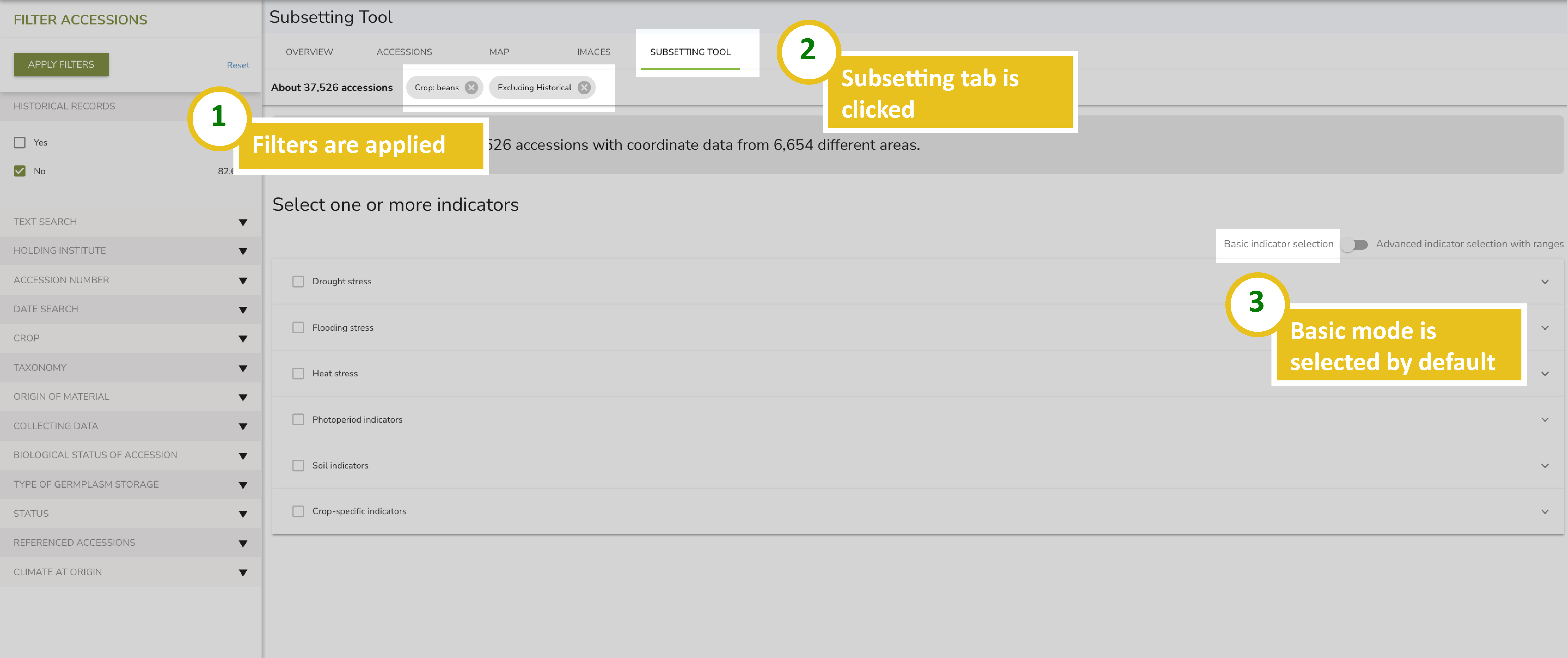
Figure 4: The Subsetting Tool interface

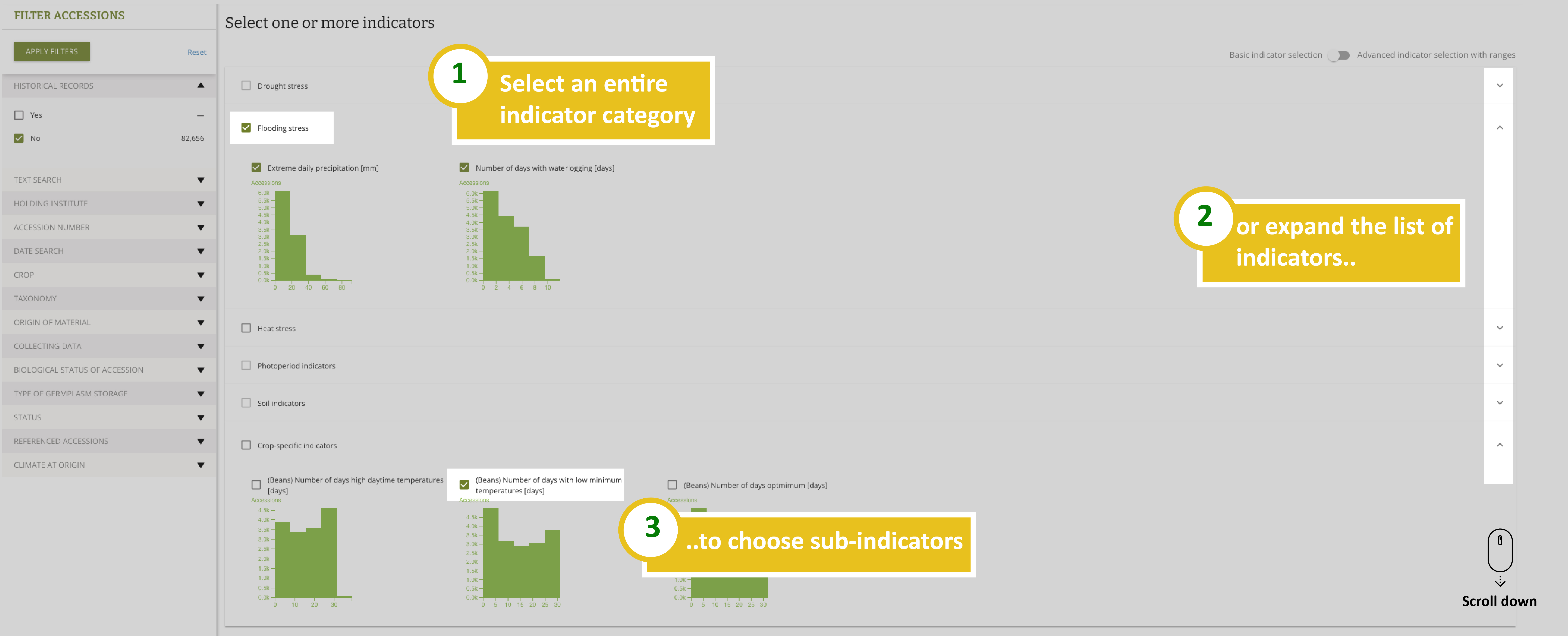
Figure 5: Selection of indicators

3. Select the number of subsets to generate using the slider, then click GENERATE to run the analysis.

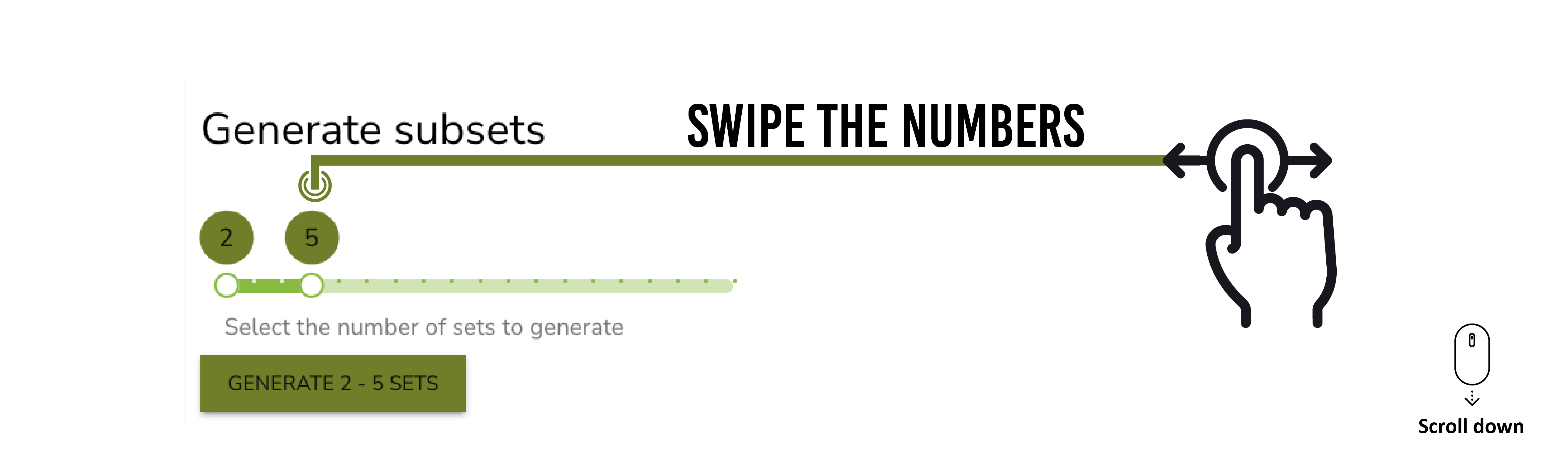
Figure 6: Generation of subsets

4. Review the results. The tool shows:
   • A pie chart with the number of accessions in each subset
   • A descriptive statistics table by indicator and subset
   • Line plots showing how each indicator behaves month by month
   • A map showing the geographical distribution of accessions

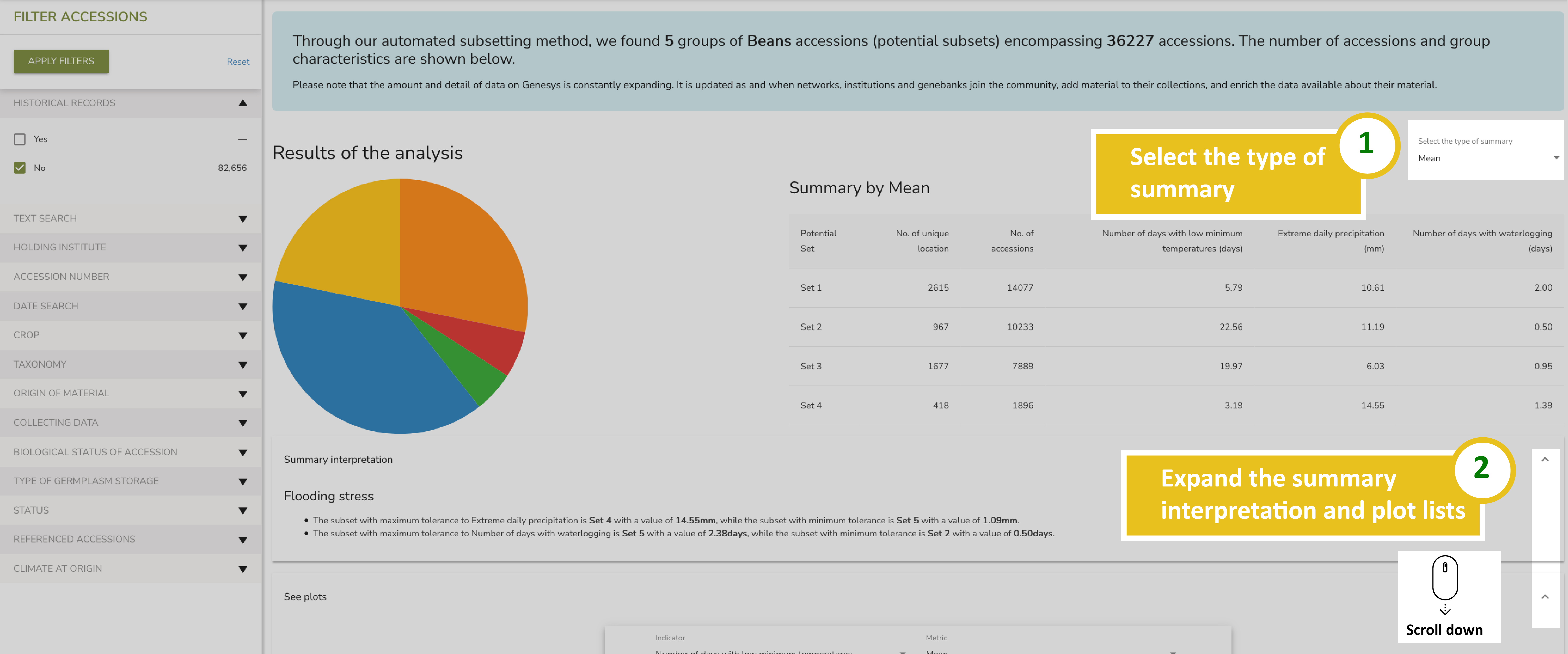
Figure 7: Results of the analysis

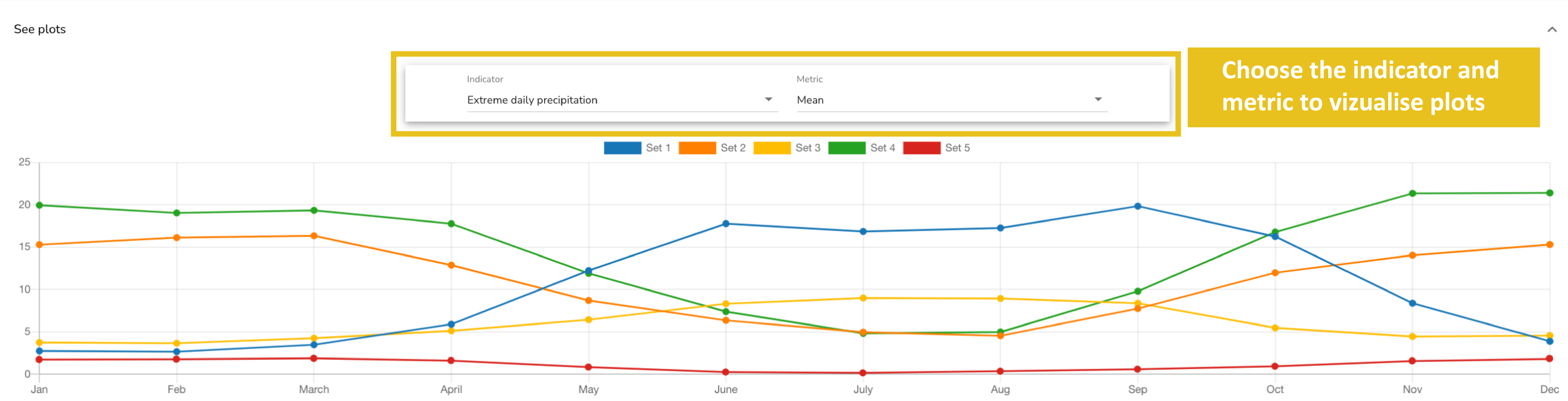
Figure 8: Mean extreme precipitation (line plot)

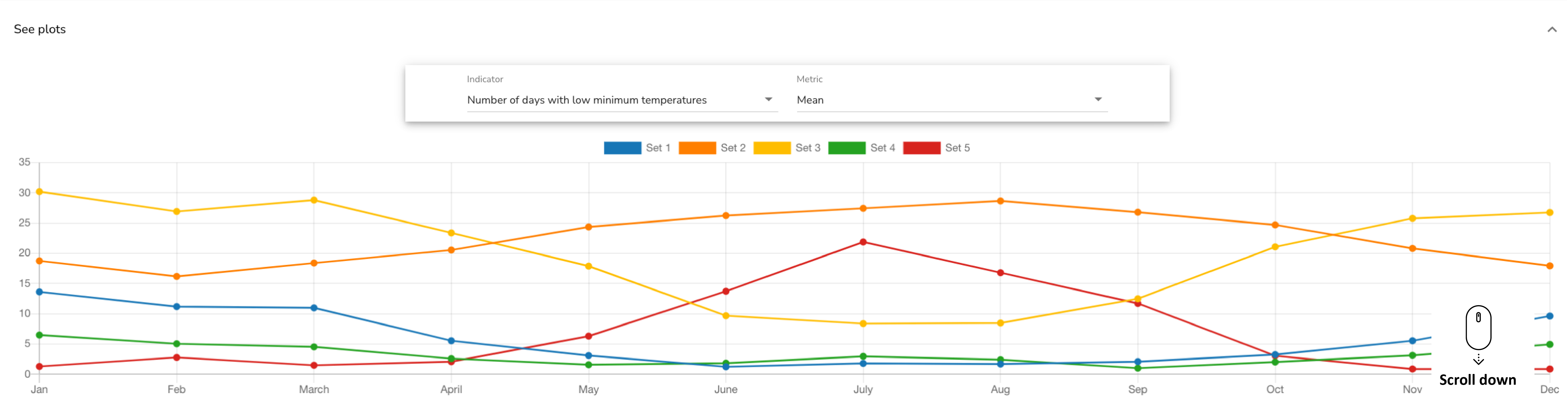
Figure 9: Mean number of days with extreme minimum temperatures (line plot)

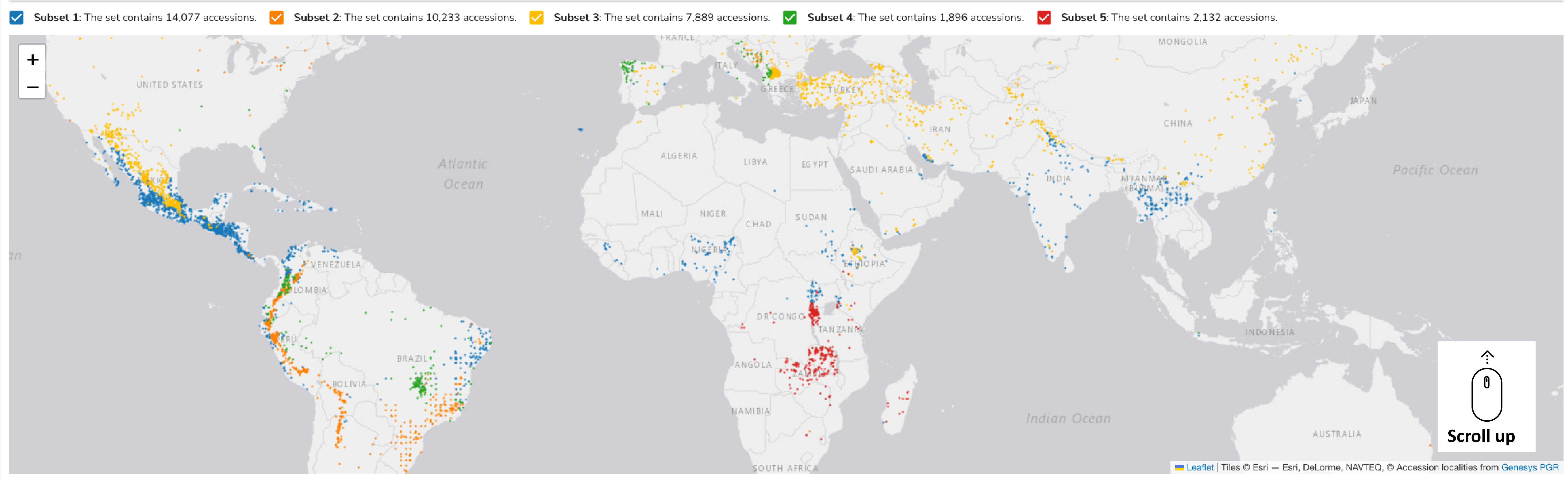
Figure 10: Geographical distribution of accessions

5. Choose the subset that most closely matches your field conditions.

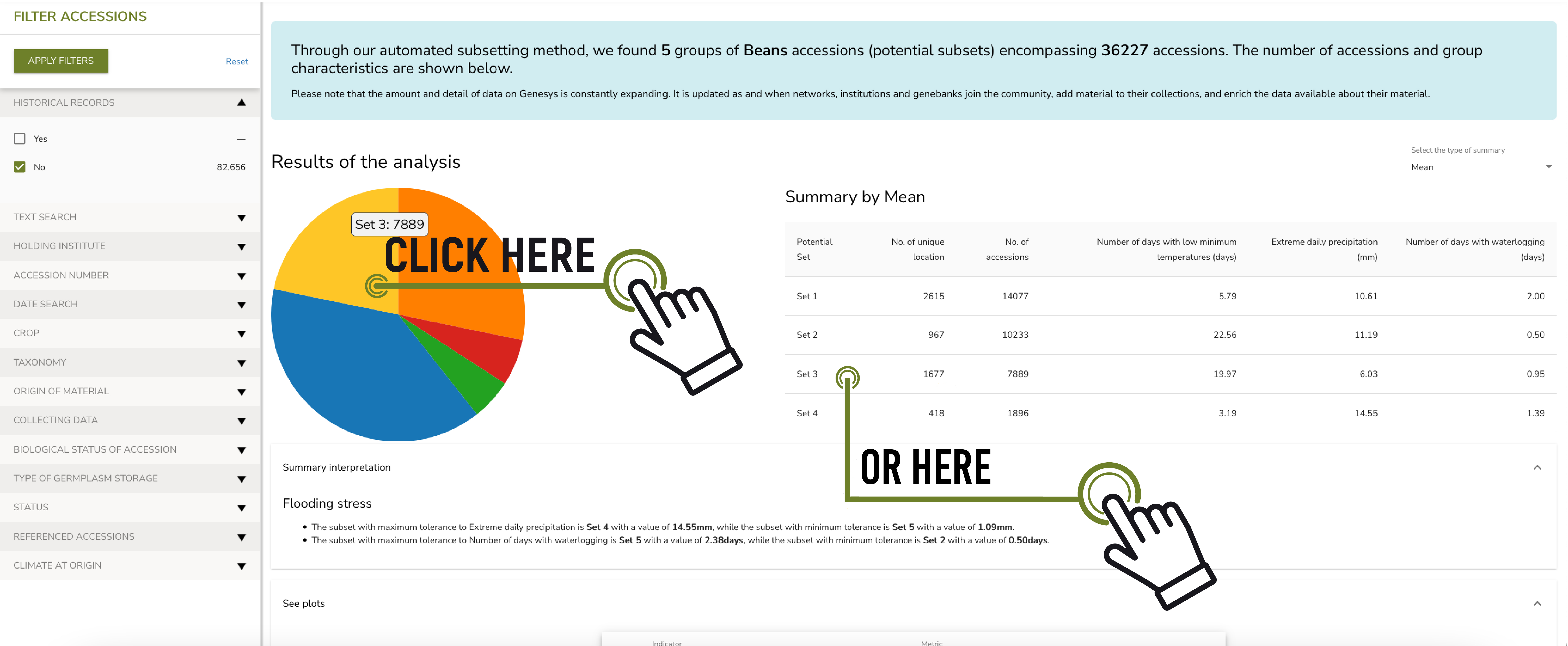
Figure 11: Selection of the subset of interest

6. After selecting a subset, view the list of accessions with their passport data.

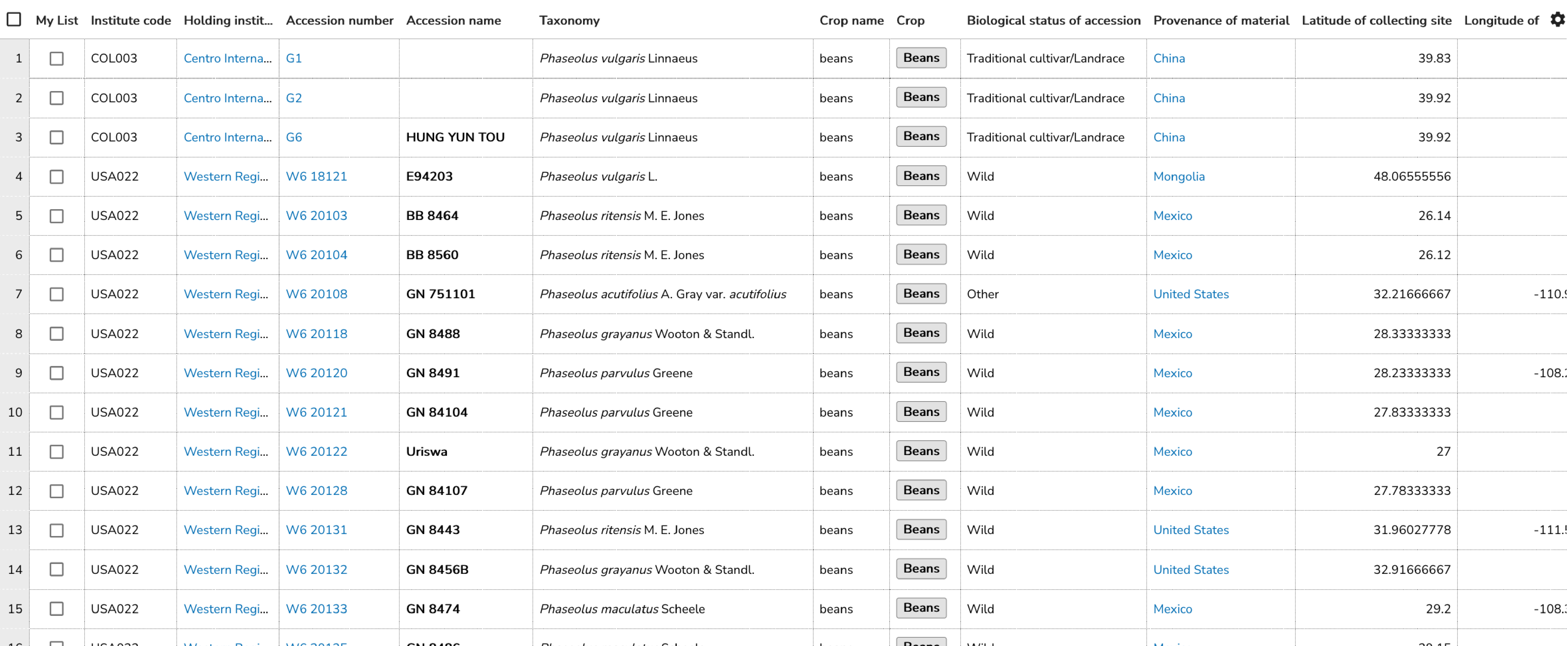
Figure 12: List of accessions resulting after the choice of the subset

If the resulting group is large (more than 50 accessions), you can filter further using the options described in the next section.

Advanced mode: Using indicator ranges

The advanced mode lets you specify exact ranges for each indicator. This is useful when you know the precise conditions of your target environment.

Example: Finding cassava for a research study

A PhD student wants to evaluate cassava accessions in a field where, from previous studies, she knows that during January to June there are high temperatures (maximum above 25 C) and very little rainfall (approximately 51 mm per month).

1. Apply a passport filter for cassava and enter the Subsetting Tool.

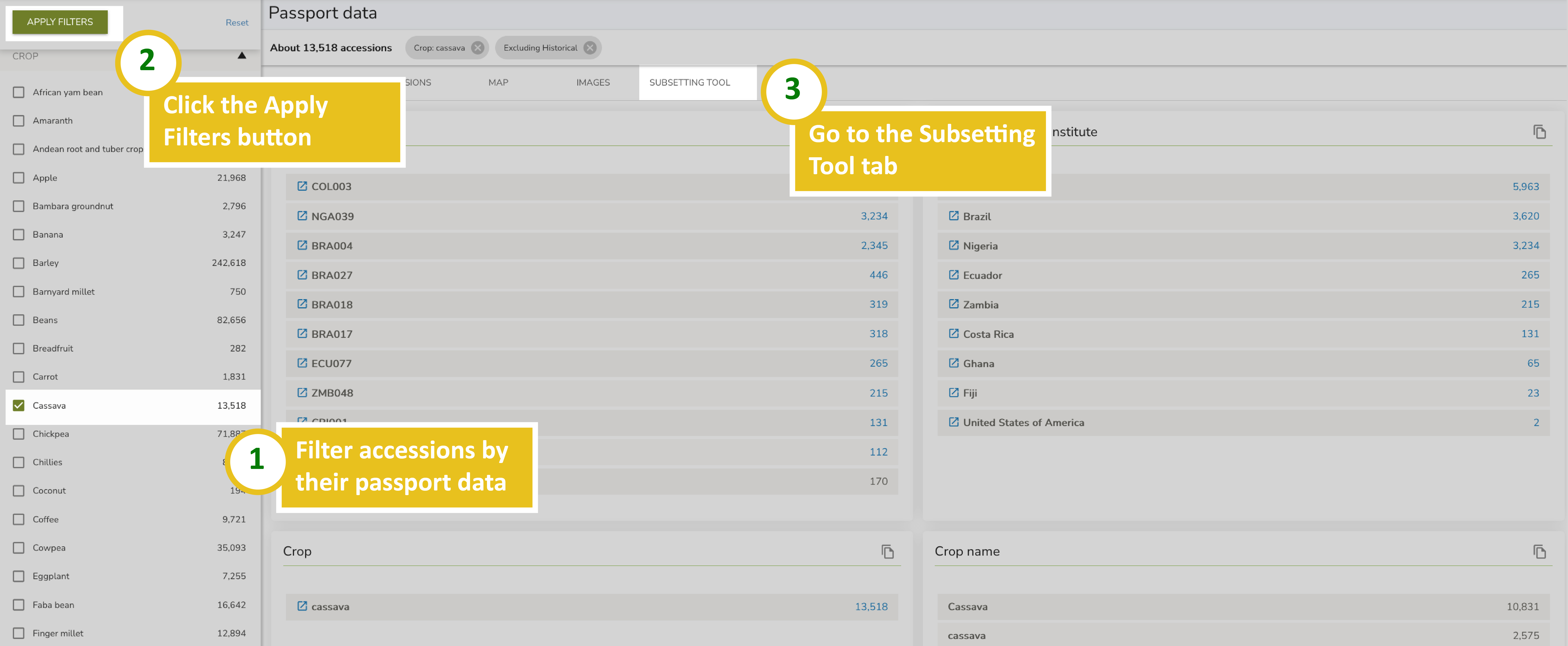
Figure 13: Steps to enter the subsetting tool with cassava selected as the crop

2. Select Advanced indicator selection with ranges.

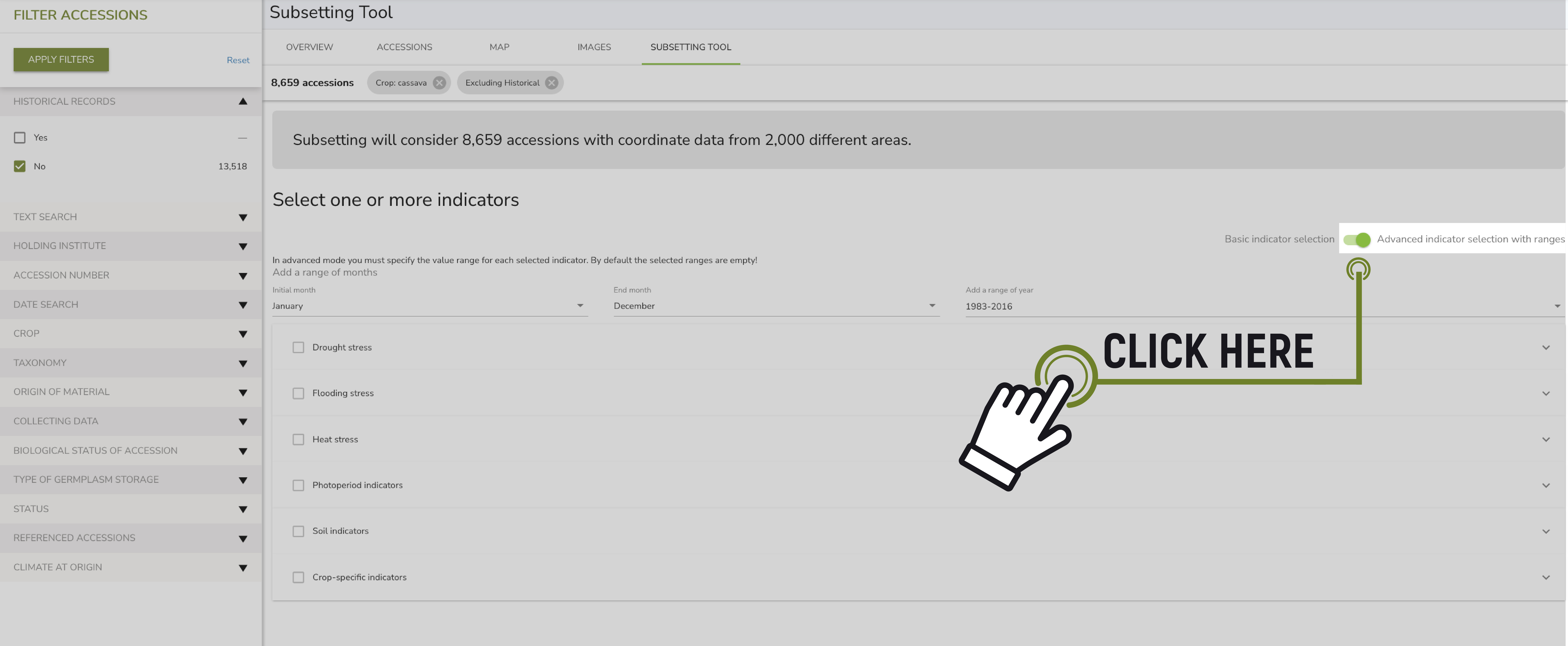
Figure 14: Activating advanced mode

3. Choose the time period for the analysis. The indicators are calculated for multiple multi-year periods (2010-2016, 2005-2016, 2000-2016, 1995-2016, 1990-2016, and 1983-2016).

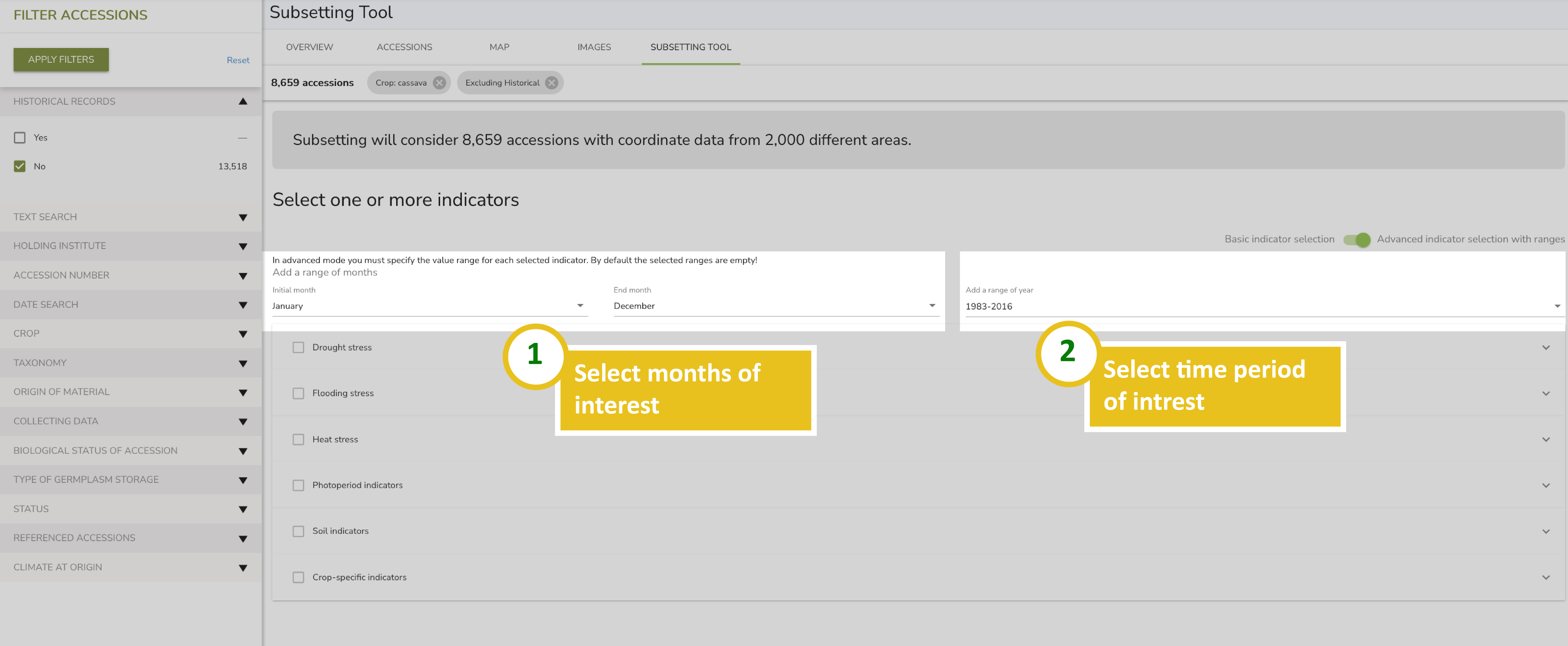
Figure 15: Selecting temporality

4. Set indicator ranges based on your known conditions:
   • Total precipitation: 0 to 51 mm
   • Average maximum temperature: greater than 25 C
   • Days with water stress: adjust as needed

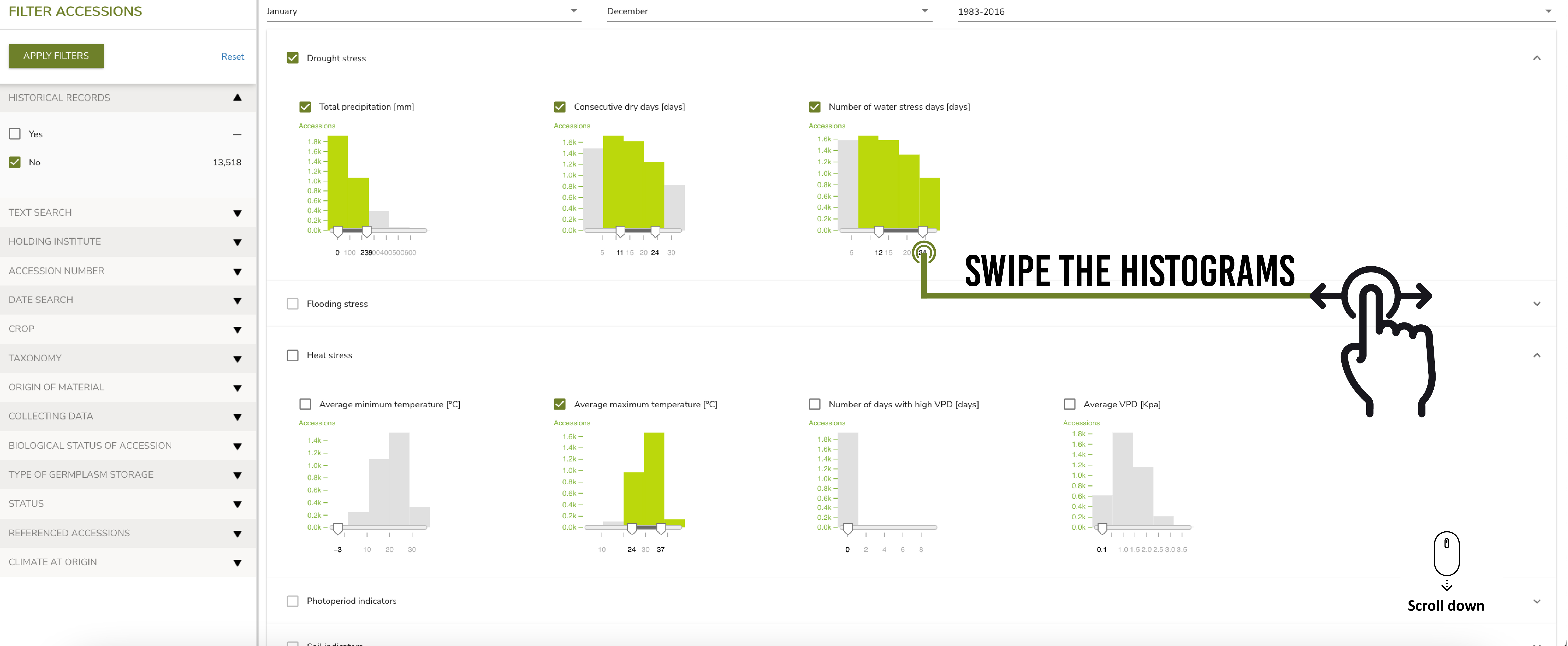
Figure 16: Selection of indicators

5. Click the filter button to generate the first subset of accessions meeting your conditions.

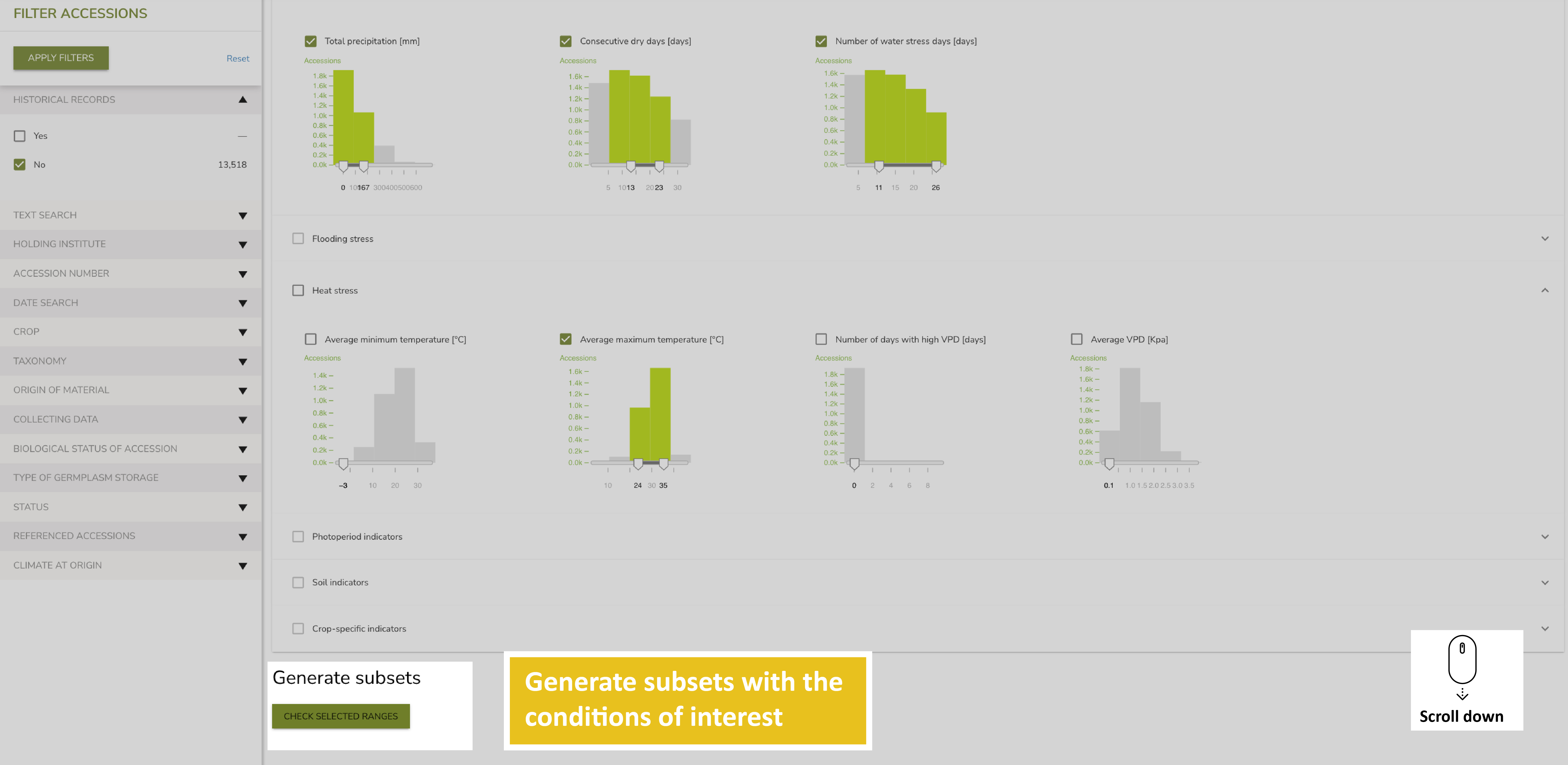
Figure 17: Filter accessions

6. Review the accessions in the Accessions tab, the map in the Map tab, and statistics in the Plots tab.

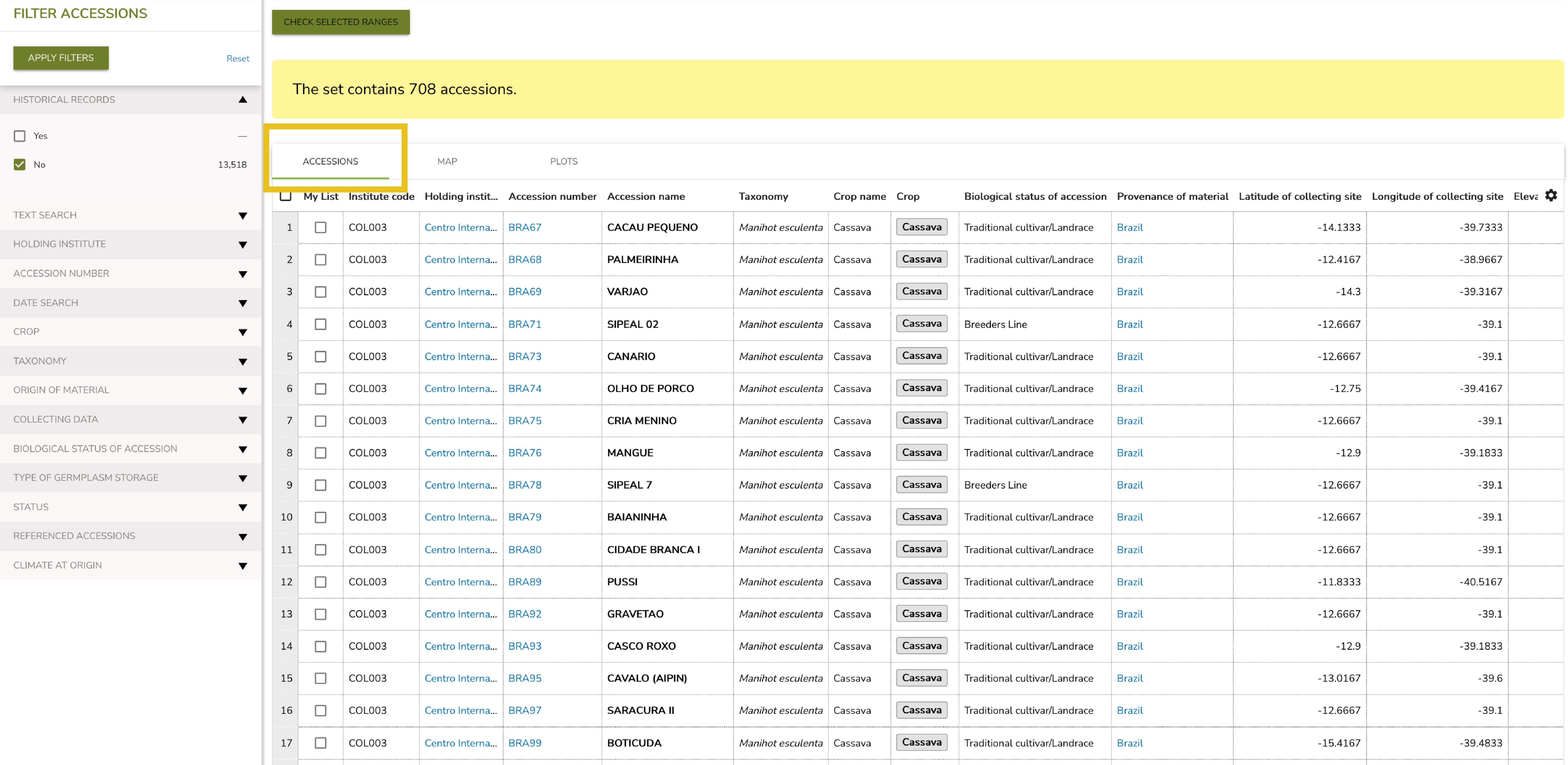
Figure 18: Accessions tab

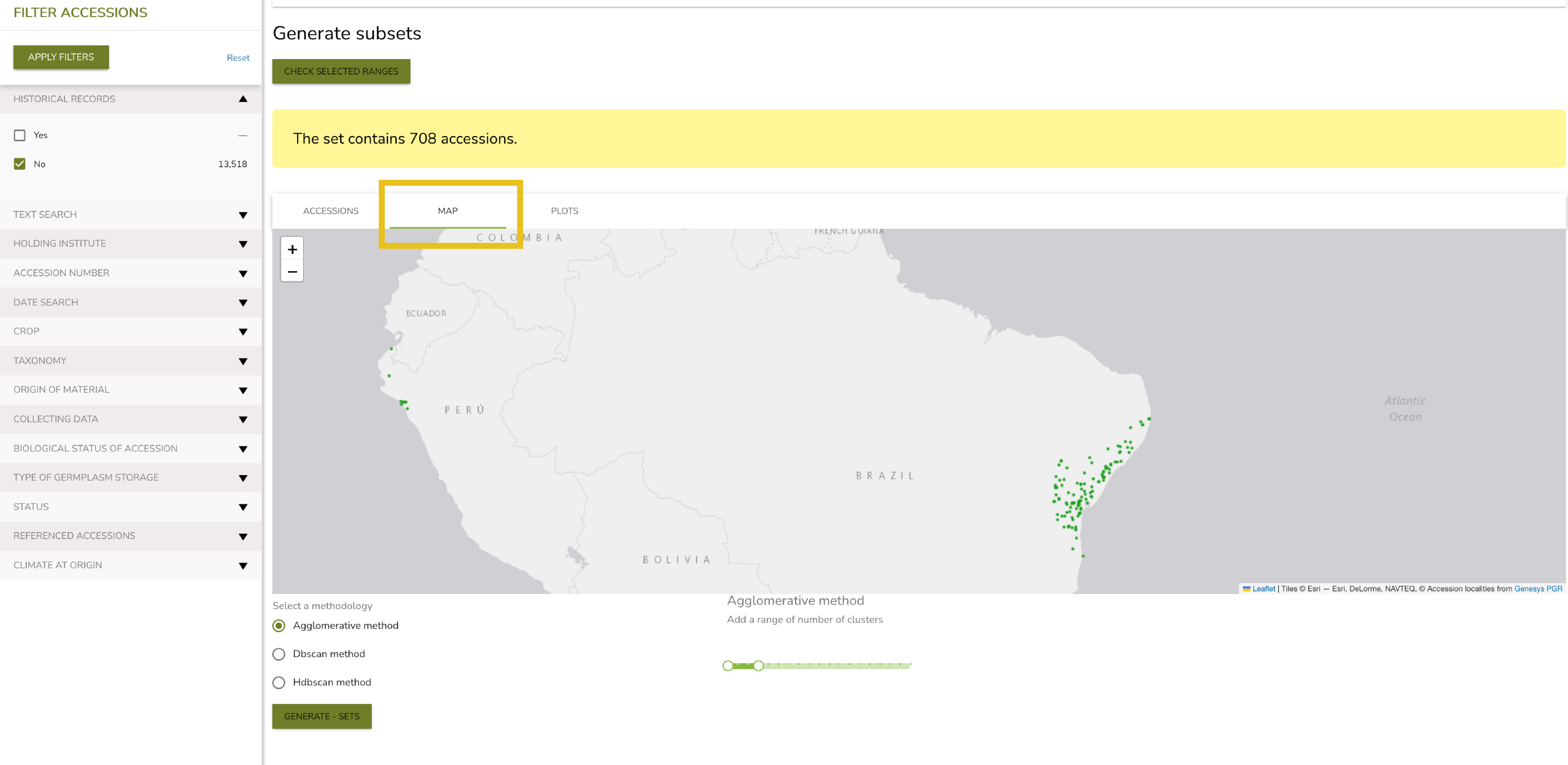
Figure 19: Geographic distribution of accessions on the Map tab

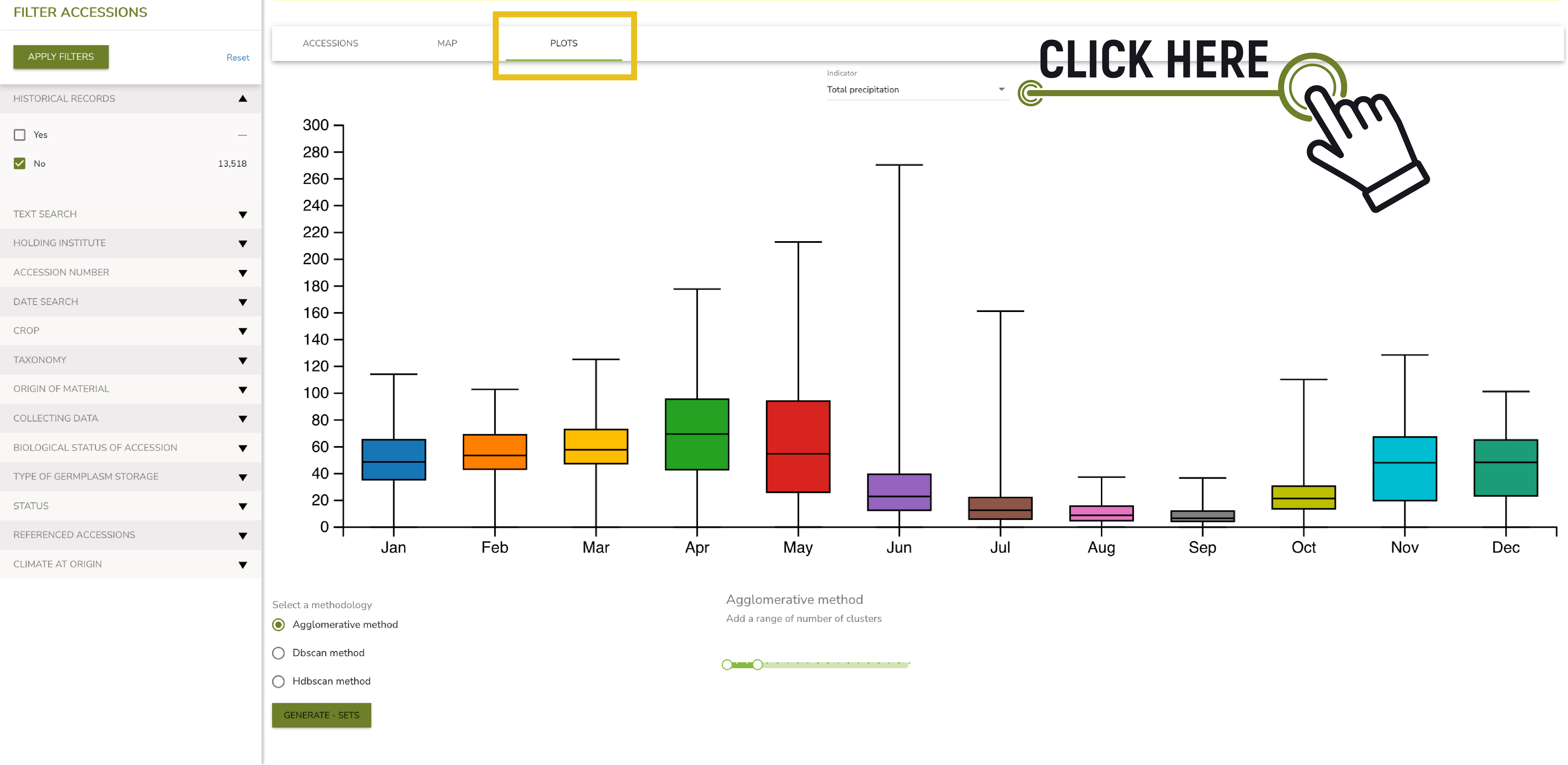
Figure 20: Plots tab

Grouping accessions with clustering methods

If you want to explore diversity within your filtered accessions, you can group them using clustering methods:

• Agglomerative method: Classic clustering where you specify the number of subsets to generate.
• DBSCAN method: Density-based clustering where you specify Epsilon (physical distance between points to join) and Minpts (minimum number of accessions per group).
• HDBSCAN method: Hierarchical density-based clustering where you specify Min_cluster_size (minimum number of points per cluster).

7. Select the agglomerative method and generate three to five subsets from the accessions.

Figure 21: Selecting the clustering method and number of subsets

8. Review the statistics, line plots, and geographical distribution to choose the subset that best matches your target conditions.

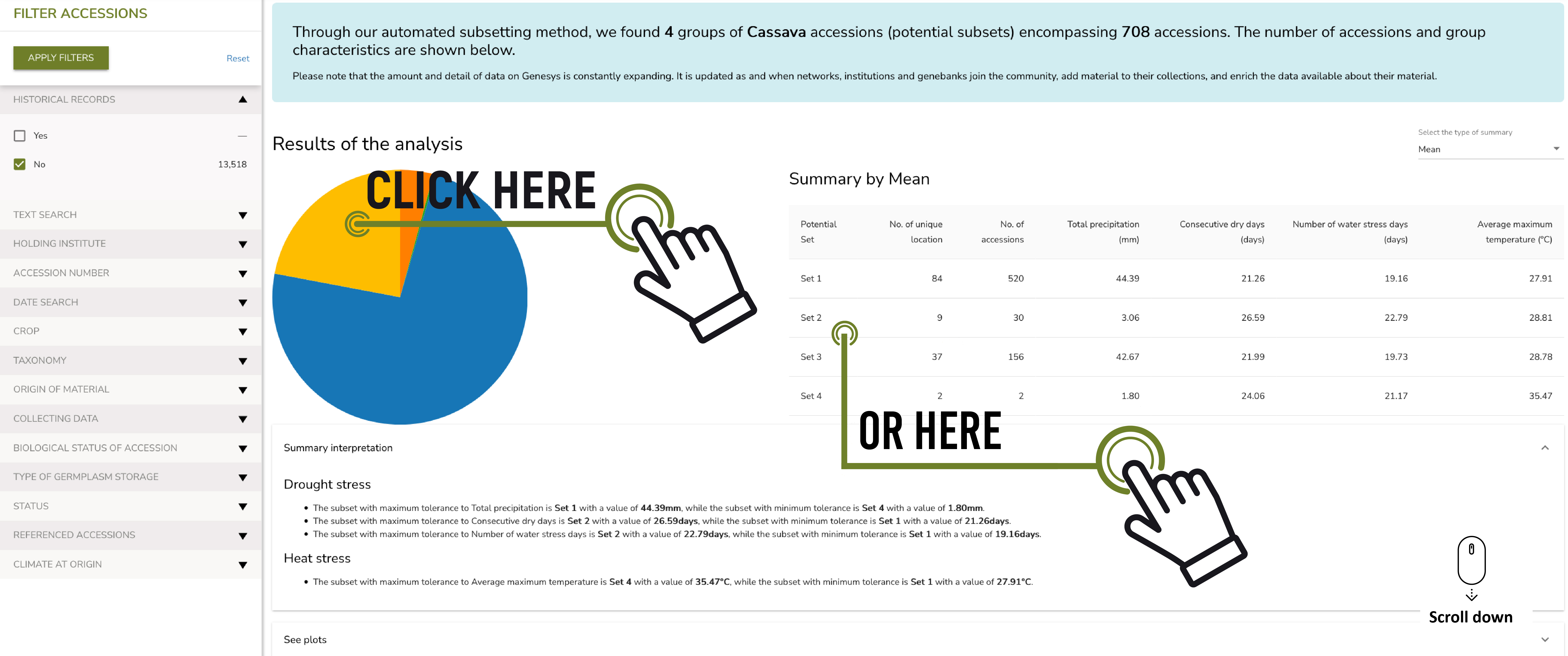
Figure 22: Selecting subset candidates

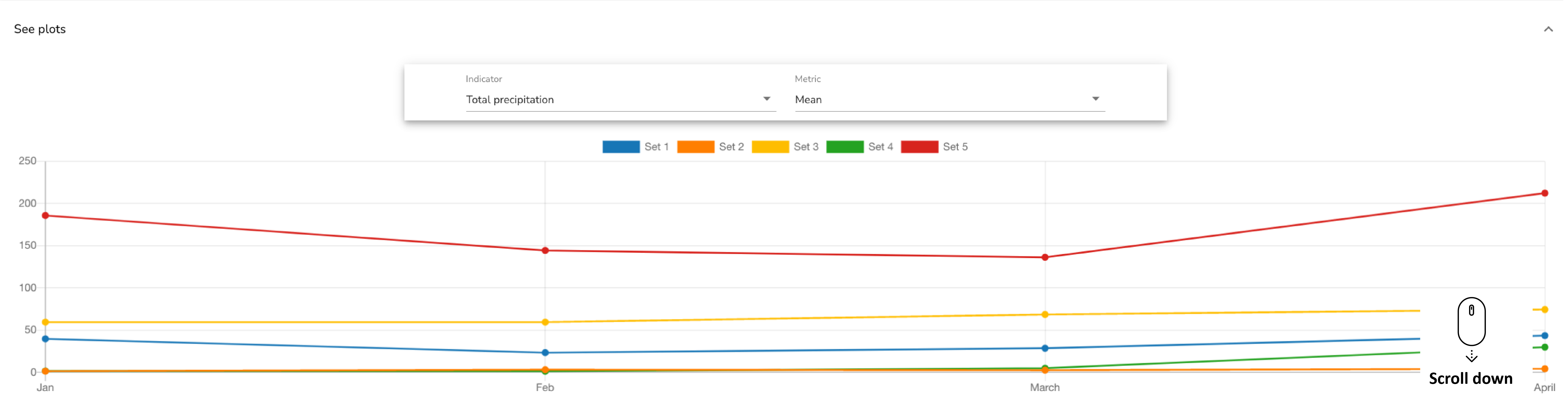
Figure 23: Line graph (mean number of consecutive dry days)

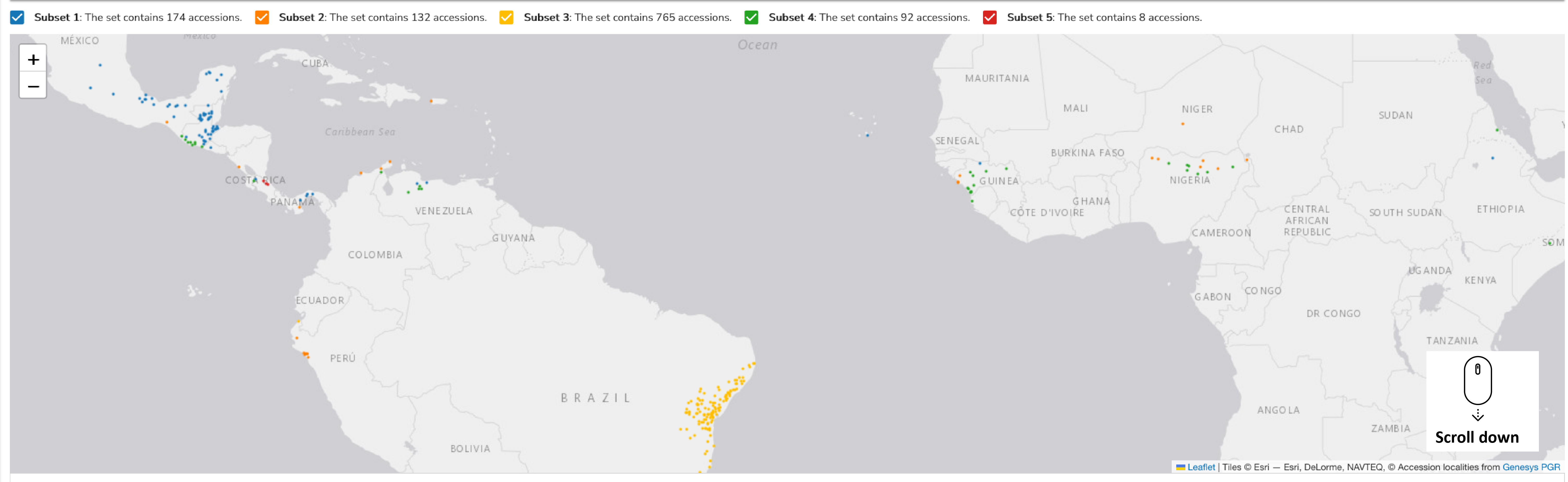
Figure 24: Geographical distribution of accessions

Based on the analysis, the student establishes that set 5 is the most suitable for her study.

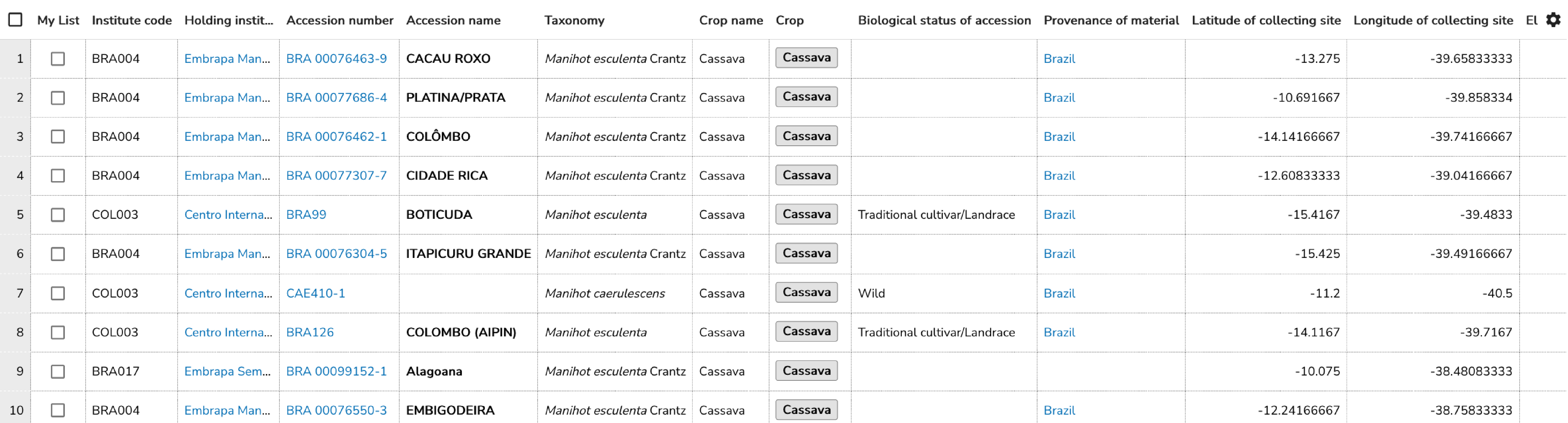
Figure 25: List of accessions resulting after the choice of a subset

Downloading accession data

If the resulting group is large (more than 50 accessions), the tool offers three options to filter and obtain a candidate subset:

• Random: Select a random sample of accessions from the results. By default, 10 accessions are selected, but you can modify this number.
• Core collection: Select the most representative accessions that capture the greatest variability of the species. This also defaults to 10 accessions.
• Manual: If you are familiar with the resulting accessions, you can select them manually.

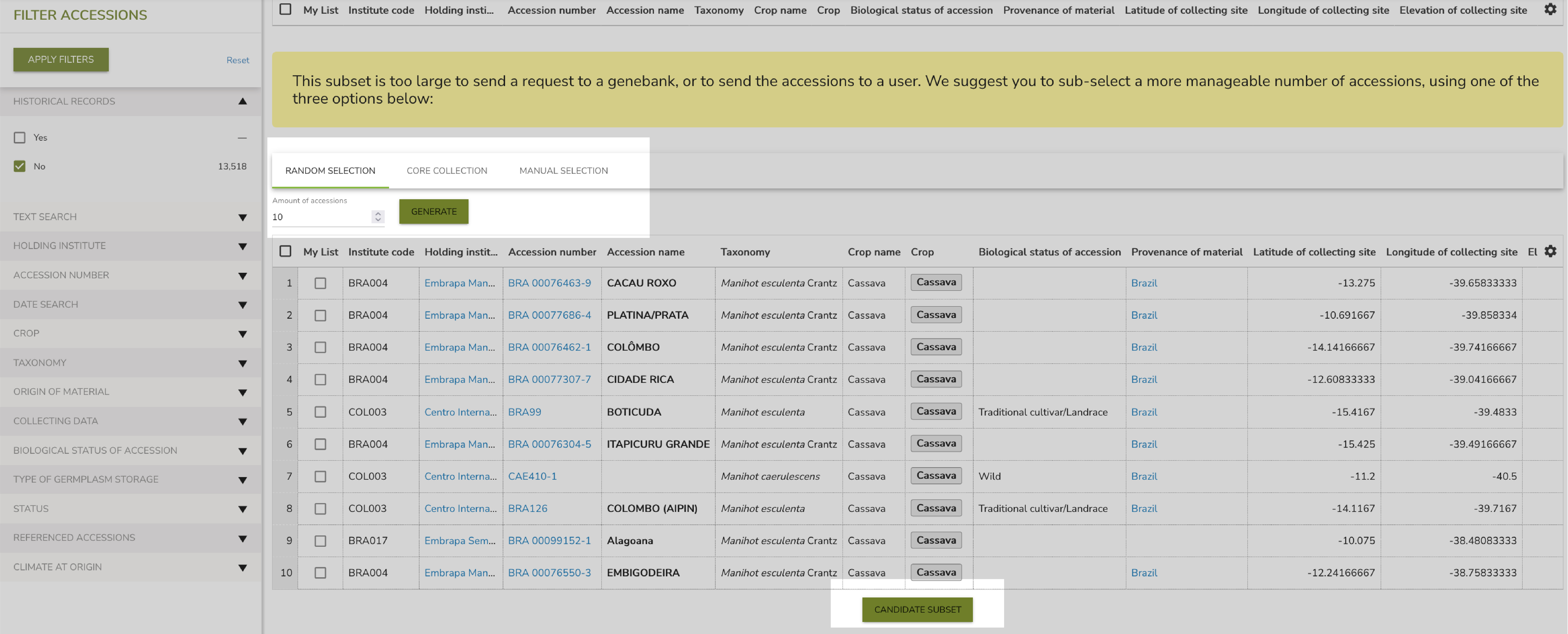
Figure 26: Choice of candidate subset

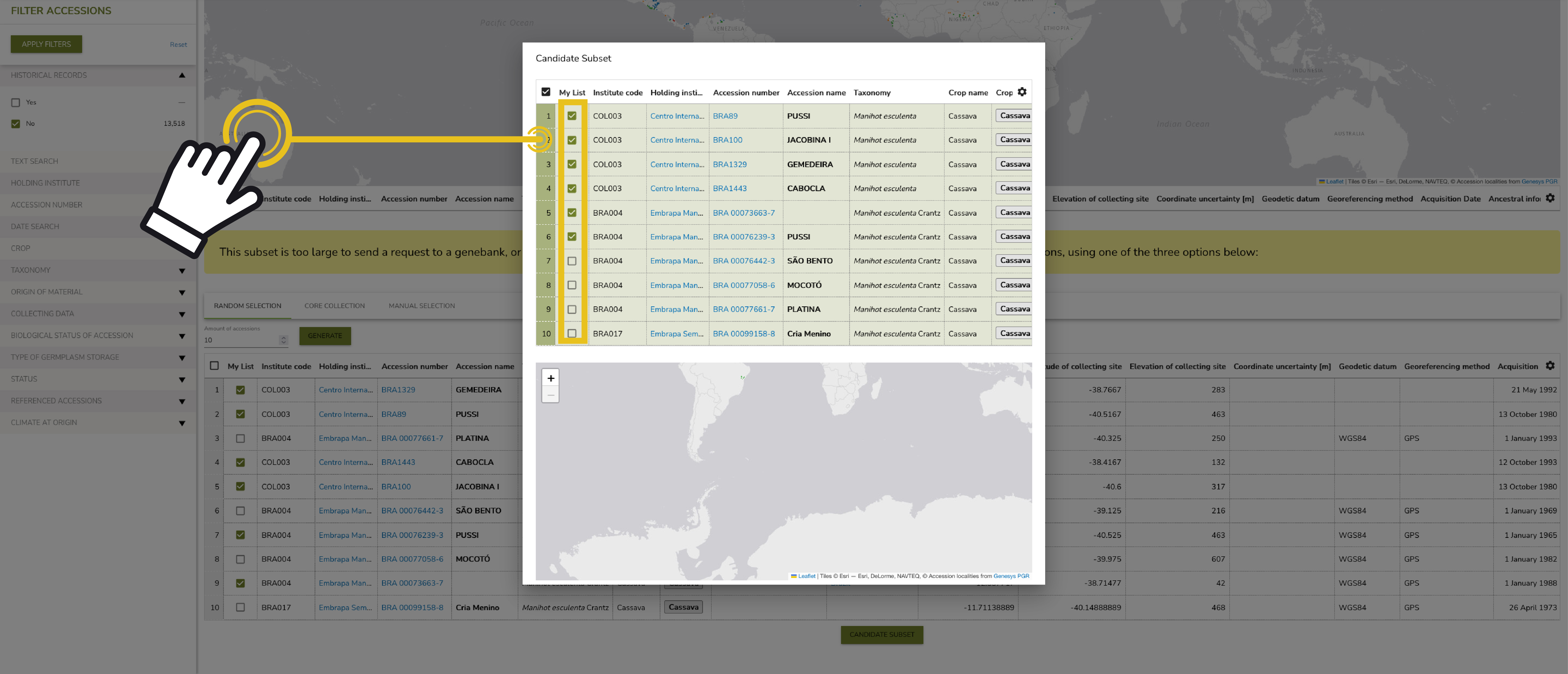
Figure 27: A candidate subset

Selected accessions are saved to your My List in your user profile, from where you can download them.

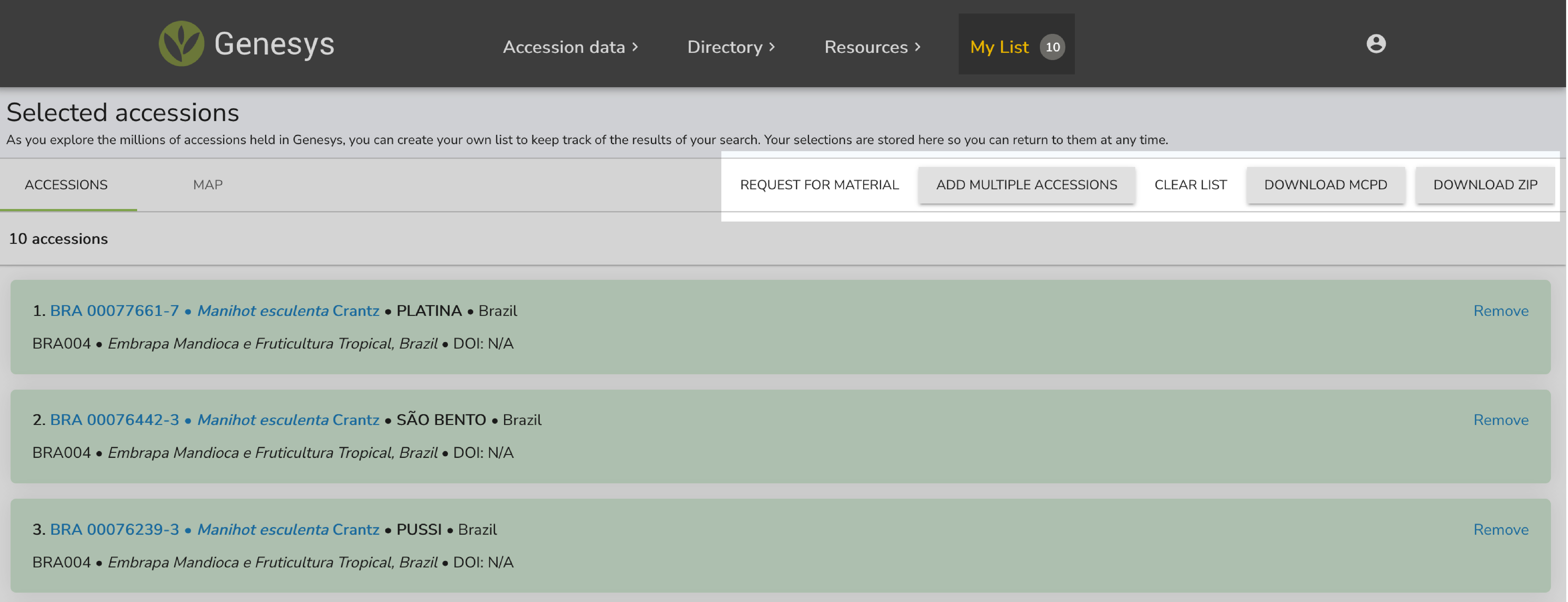
Figure 28: Downloading selected accessions from the candidate subset

Resources

Generic indicators

The following datasets provide the agroclimatic indicators used by the Subsetting Tool:

• North America
• South America
• Asia
• Europe
• Oceania
• Africa

Crop-specific indicators

Crop-specific indicators are available for these crops: bean, cassava, banana, wheat, maize, potato, sweet potato, rice, barley, sorghum, pearl millet, cowpea, yam, soybean.

• South America
• Oceania
• Europe
• Africa
• North America

Bibliography

• Hengl, T. et al. (2017). SoilGrids250m: Global gridded soil information based on machine learning. PLoS one, 12(2), e0169748.
• Funk, C. et al. (2015). The climate hazards infrared precipitation with stations: a new environmental record for monitoring extremes. Scientific data, 2(1), 1-21.
• Verdin, A. et al. (2020). Development and validation of the CHIRTS-daily quasi-global high-resolution daily temperature data set. Scientific Data, 7(1), 303.
• Ruane, A. C. (2021). AgMERRA and AgCFSR Climate Forcing Datasets for Agricultural Modeling.